In this post you can find a Matlab code for constructing digital nets on 
![L_2([0,1])](https://s0.wp.com/latex.php?latex=L_2%28%5B0%2C1%5D%29&bg=ffffff&fg=333333&s=0&c=20201002) . In this post we discuss the rate of decay of the Walsh coefficients when the function has bounded variation of fractional order
. In this post we discuss the rate of decay of the Walsh coefficients when the function has bounded variation of fractional order  and we investigate pointwise convergence of the Walsh series and pointwise convergence of the Walsh series to the function. We consider only Walsh functions in base
  although the results can be generalized to Walsh functions over groups. Information on Walsh functions over groups can be found in
  be an arbitrary
 ![\boldsymbol{c}:[a,b]\to\mathbb{R}^n,](https://s0.wp.com/latex.php?latex=%5Cboldsymbol%7Bc%7D%3A%5Ba%2Cb%5D%5Cto%5Cmathbb%7BR%7D%5En%2C&bg=ffffff&fg=333333&s=0&c=20201002) and the curve
and the curve  which is the image of
  given by
 ![\{\boldsymbol{c}(t) \in \mathbb{R}^n: t\in [a,b]\}.](https://s0.wp.com/latex.php?latex=%5C%7B%5Cboldsymbol%7Bc%7D%28t%29+%5Cin+%5Cmathbb%7BR%7D%5En%3A+t%5Cin+%5Ba%2Cb%5D%5C%7D.&bg=ffffff&fg=333333&s=0&c=20201002) Here we shall discuss parameterised curves. Hence, for instance, the parameterised curve
Here we shall discuss parameterised curves. Hence, for instance, the parameterised curve 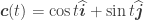 with
with  is a circle traversed twice and has therefore length
  whereas its image is just a circle which has length
Search
Categories
Archives
Subscribe to feed

-
Join 38 other subscribers
Conferences
Diversions
Misc
Tags
best approximation lemma bounded variation Cauchy Schwarz inequality completely uniformly distributed complete orthonormal system continuous convergence differentiable differential Differential form digital net Dirichlet kernel discrepancy theory Divergence theorem Duality Theory for Digital Nets even function fast component by component Fejér kernel Fourier series Fourier series applet Fourier series applications Fourier series background Fourier series examples fundamental theorem of line integrals Gibbs sampler Green's theorem Green's theorem in normal form Green's theorem in tangential form heat equation Higher order digital net higher order digital sequence higher order polynomial lattice rule higher order Sobol sequence ICIAM 2011 Korobov space lattice rule limit line integral L_2 space Markov chain Monte Carlo mean square convergence mean square convergence of Fourier series multiple lightswitches Norm numerical integration numerical integration over R^s odd function one sided limit orientation of curve Parseval's identity periodic functions piecewise continuous piecewise differentiable polynomial lattice rule Propagation Rule pseudo random numbers Pythagorean theorem quasi-Monte Carlo randomised quasi-Monte Carlo scalar line integral sequence of functions Several Variable Calculus slice sampler Sobol sequence Stokes Theorem Surface integrals tiling tractability triangle inequality trigonometric polynomial variation vector field Walsh function Walsh model Weierstrass testRecent Comments
Pages
Meta