In this blog entry you can find lecture notes for Math2111, several variable calculus. See also the table of contents for this course. This blog entry printed to pdf is available here.
Work integral
Previously we considered integrals of a function  (n=2,3) over a curve
  . We now turn to integrating vector fields
  where
where  or
or  . These integrals can be motivated by calculating the work done by a force on a particle along some curve .
In the simplest case, the work  done a force
  acting on an object which moves along a straight line is given by
where the object is displaced in the direction of the vector  with distance
  .
.
In a more general setting, the object moves along a curve ![\boldsymbol{r}:[a,b]\to\mathbb{R}^n](https://s0.wp.com/latex.php?latex=%5Cboldsymbol%7Br%7D%3A%5Ba%2Cb%5D%5Cto%5Cmathbb%7BR%7D%5En&bg=ffffff&fg=333333&s=0&c=20201002) . One way to arrive at a formula for calculating the work done by a force
. One way to arrive at a formula for calculating the work done by a force  along
along  is to take the component of in the tangential direction on each point on the curve and integrate this quantity using a scalar line integral. The tangential direction on the curve at a point
  is given by
  and a unit vector in tangential direction is given by

where  denotes the Euclidian norm and where we assume that
  for all
 ![t\in[a,b].](https://s0.wp.com/latex.php?latex=t%5Cin%5Ba%2Cb%5D.&bg=ffffff&fg=333333&s=0&c=20201002) Hence the component of in the direction of the tangent to the curve at a point is given by
Hence the component of in the direction of the tangent to the curve at a point is given by

This is now a scalar valued function which can be integrated using the scalar line integral. We thus obtain that the work done is given by
where we used  .
.
Line integral
We can now formally define line integrals of vector fields over some curve.
Line Integral
Let or . Let be a continuously differentiable curve and let  be a continuous vector field, where we assume that
 ![\{\boldsymbol{r}(t):t\in[a,b]\} \subseteq D.](https://s0.wp.com/latex.php?latex=%5C%7B%5Cboldsymbol%7Br%7D%28t%29%3At%5Cin%5Ba%2Cb%5D%5C%7D+%5Csubseteq+D.&bg=ffffff&fg=333333&s=0&c=20201002) Then we define
Then we define  , the line integral of along , by the formula

Notice that we do not need the assumption that  for all
 ![t\in[a,b]](https://s0.wp.com/latex.php?latex=t%5Cin%5Ba%2Cb%5D&bg=ffffff&fg=333333&s=0&c=20201002) . This can be shown by setting up Riemann sums as in the case for scalar line integrals. (This makes a difference in some cases. For example, for
. This can be shown by setting up Riemann sums as in the case for scalar line integrals. (This makes a difference in some cases. For example, for  we get
  , and this cannot be avoided using a different parameterisation.)
Line integrals are written in various forms. For instance, let  and
and  . Then the line integral is also written as

There also exist analogous ways for writing line integrals for the two-dimensional case.
Example
Let  for
for  and
and  . Then from the parameterisation of the curve we have
 and
and  Hence
Hence 
 and
and  Further
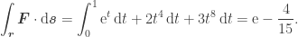
 Hence
Hence

Some properties of line integrals
Let  be continuous vector fields and let
  be a constant.
-

-
- Let be a smooth curve and let
 denote the same curve but with the orientation reversed. Then
- Let be a union of
 smooth curves
  , then
Line integrals in the plane in normal form
We defined line integrals by integrating the tangential component of a vector field over a curve . In the plane it is also meaningful to compute the orthogonal component of the vector field along some curve . Let ![\boldsymbol{r}:[a,b]\to\mathbb{R}^2](https://s0.wp.com/latex.php?latex=%5Cboldsymbol%7Br%7D%3A%5Ba%2Cb%5D%5Cto%5Cmathbb%7BR%7D%5E2&bg=ffffff&fg=333333&s=0&c=20201002) with
with  be a curve and let
  be a unit normal vector to the curve at the point which is obtained by turning the unit tangent vector
  by
by  clockwise, then this line integral is given by